The first brachiation robot work was done by Saito, Fukada et al. [Saito1994swing][Saito1993swing] in the Robotics Lab at Nagoya University. Publications on Brachiator III aparently in F. Sato 97 Artificial life V and Y. Hasegawa Advances in artifical life 1999
Cybernetics: The scientific study of control and communication in the animal and the machine. Norbert Wiener 1948
... which I call Cybernétique, from the word $\kappa\nu\beta\epsilon\rho\nu\varepsilon\tau\iota\chi\eta$ which at first (taken in a limited sense) is the art of governing a vessel but (even among the Greeks) extends to the art of governing in general.[ampere38:essai] André-Marie AmpèreThe ancient Greek word kybernetikos ("good at steering"), refers to the art of the helmsman.
Latin word guberno/gubernãre that is the root of words for government comes from the same Greek word that gives rise to cybernetics.
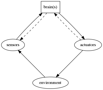
The posession of a brain allows humans, animals and (to some extent) robots to have a meaningful interaction in a complex environment. Intelligence may be observed from the way we react in this environment but (as shown in figure below), sense our environment and use this information to update internal models we have of the world. We react to this information via our understanding of the behaviour of our internal models and operate through muscles to enable us to alter our enviromnent to our benefit.
Other relevant concepts
Highly recommended Ted Talk (https://www.ted.com/talks/daniel_wolpert_the_real_reason_for_brains) Daniel Wolpert. The real reason for brains. March 2014
A system is an object that we would like to study, control and affect the behavior.
A model is the knowledge of the properties of a system. It is necessary to have a model of the system in order to solve problems such as control, signal processing, system design. Sometimes the aim of modelling is to aid in design. Sometimes a simple model is useful for explaining certain phenomena and reality.
A model may be given in any one of the following forms:
A value $y(t)$ exists at all points values of $t$ (or more usually all points in $t\ge 0$)
This should also be true of all derrivatives of $y$
Formed as output y(t) responding to input u(t) to a system g(t)
\[ y(t)=\int_{-\infty}^\infty u(\tau) g(t-\tau) d\tau \]This is convolution and can be considered graphically as follows[Wang11:_e101]
Laplace transformed versions
\[ Y(s)=G(s)U(s) \]Frequency domain and frequency response (Ying Zheng)
A value $y(n)$ exists only at specific times, that is at all positive integer values of $n$. It may be convenient to occasionally include 0 or negative integers in $n$.
Tend to be defined in terms of a delay operator $q^{-1}$ such that for a sequence $u(i)$ the operator delays each value by one timestep, i.e. $q^{-1}u(i)=u(i-1)$. The $q$ operator is interchangeable with the $z$ transform.
Formed as output y(n) responding to input u(n) to a system g(n) where n is an integer, i.e. the output does not exist for any time $t\ne n$
\[ y(n)=\sum_{i=-\infty}^\infty u(i) g(n-i) \]If $y=f(u(t))$ is a system (or function) with an input $u(t)$ that can change with time $t$ then the system can be considered as linear if
\[ y'=f(a u(t))=a y \]for some constant scalar value $a$.
This applies also to the vector form i.e. if $\vec{y}=f(\vec{u})$ then the system can be considered as linear if
\[ a\vec{y}=f(a\vec{u}) \]If $y(t)=f(u(t))$ for input $u$ at time $t$ then the system can be considered as time variant if for some constant scalar value $\tau$ (or $a$) $y'(t)=f(u(t+\tau))=y(t+\tau)$ for some constant scalar value $a$ Again this applies also to the vector form
The concept of state space has two benefits, first it allows a system to be described as a vector of states such as position, velocity, voltage, current etc. Second it allows the equations (both linear and non linear) to be written as a single level of differentiation.
The general form for a state space with states $\vec{x}(t)$, inputs $\vec{u}(t)$ and outputs $y(t)$ is
\begin{align} \dot{\vec{x}}&=f(\vec{x},\vec{u},t)\\ \vec{y}&=g(\vec{x},\vec{u},t) \label{eq:nonlinCD} \end{align}with input $\vec{u}$, output $\vec{y}$ and states $\vec{x}$. All variables are assumed to be a function of $t$.
Linear state space equations are often written with the ABCD notation
\begin{align} \dot{\vec{x}}&= A \vec{x} +B\vec{u}\\ \vec{y}&= C\vec{x}+D\vec{u} \label{eq:linCD} \end{align}With constant matrices $A,B,C,D$
Often, in both linear and non-linear versions, the equations above are simplifed to $\vec{y}= C\vec{x}$ with C being an identity matrix.It is often. necessary to approximate a non-linear system with a locally equivalent linear system. Then many of the tools for linear systems can be used as long as things don't change too significantly.
Linearisation occurs around a stationary operating point, and is best explained with Taylor's theorem.
Any function $f(x)$ can be approximated around an stationary operating point $a$ as the Taylor's expansion so that
\[ f(x)=f(a)+f'(a)(x-a)+\frac12 f''(a)(x-a)^2 ... \]Note the notation where again $f'$ means differentiating. We ignore higher orders so for a first order system we have
\[ \dot{x}=f(x)\approx f(a)+f'(a)x-f'(a)a=c_1+c_2 x \]where $c_1=f(a)-f'(a)a$ and $c_2=f'(a)$
This same concept can be extended into vector forms, i.e. given $\dot{\vec{x}}=f(\vec{x})$ we can find a linear approximation where $\dot{\vec{x}} = A \vec{x}$